
Distance Calculator
The calculators below can be used to find the distance between two points on a 2D plane or 3D space. They can also be used to find the distance between two pairs of latitude and longitude, or two chosen points on a map.
2D Distance Calculator
Use this calculator to find the distance between two points on a 2D coordinate plane.
3D Distance Calculator
Use this calculator to find the distance between two points on a 3D coordinate space.
Distance Based on Latitude and Longitude
Use this calculator to find the shortest distance (great circle/air distance) between two points on the Earth's surface.
Distance on Map
Click the map below to set two points on the map and find the shortest distance (great circle/air distance) between them. Once created, the marker(s) can be repositioned by clicking and holding, then dragging them.
Distance in a coordinate system
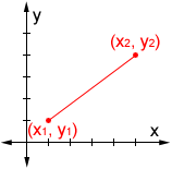
Distance in a 2D coordinate plane:
The distance between two points on a 2D coordinate plane can be found using the following distance formula
d = √(x2 - x1)2 + (y2 - y1)2
where (x1, y1) and (x2, y2) are the coordinates of the two points involved. The order of the points does not matter for the formula as long as the points chosen are consistent. For example, given the two points (1, 5) and (3, 2), either 3 or 1 could be designated as x1 or x2 as long as the corresponding y-values are used:
Using (1, 5) as (x1, y1) and (3, 2) as (x2, y2):
| d = | √(3 - 1)2 + (2 - 5)2 |
| = | √22 + (-3)2 |
| = | √4 + 9 |
| = | √13 |
Using (3, 2) as (x1, y1) and (1, 5) as (x2, y2):
| d = | √(1 - 3)2 + (5 - 2)2 |
| = | √(-2)2 + 32 |
| = | √4 + 9 |
| = | √13 |
In either case, the result is the same.
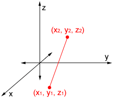
Distance in a 3D coordinate space:
The distance between two points on a 3D coordinate plane can be found using the following distance formula
d = √(x2 - x1)2 + (y2 - y1)2 + (z2 - z1)2
where (x1, y1, z1) and (x2, y2, z2) are the 3D coordinates of the two points involved. Like the 2D version of the formula, it does not matter which of two points is designated (x1, y1, z1) or (x2, y2, z2), as long as the corresponding points are used in the formula. Given the two points (1, 3, 7) and (2, 4, 8), the distance between the points can be found as follows:
| d = | √(2 - 1)2 + (4 - 3)2 + (8 - 7)2 |
| = | √12 + 12 + 12 |
| = | √3 |
Distance between two points on Earth's surface
There are a number of ways to find the distance between two points along the Earth's surface. The following are two common formulas.
Haversine formula:
The haversine formula can be used to find the distance between two points on a sphere given their latitude and longitude:
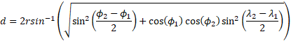
In the haversine formula, d is the distance between two points along a great circle, r is the radius of the sphere, ϕ1 and ϕ2 are the latitudes of the two points, and λ1 and λ2 are the longitudes of the two points, all in radians.
The haversine formula works by finding the great-circle distance between points of latitude and longitude on a sphere, which can be used to approximate distance on the Earth (since it is mostly spherical). A great circle (also orthodrome) of a sphere is the largest circle that can be drawn on any given sphere. It is formed by the intersection of a plane and the sphere through the center point of the sphere. The great-circle distance is the shortest distance between two points along the surface of a sphere.
Results using the haversine formula may have an error of up to 0.5% because the Earth is not a perfect sphere, but an ellipsoid with a radius of 6,378 km (3,963 mi) at the equator and a radius of 6,357 km (3,950 mi) at a pole. Because of this, Lambert's formula (an ellipsoidal-surface formula), more precisely approximates the surface of the Earth than the haversine formula (a spherical-surface formula) can.
Lambert's formula:
Lambert's formula (the formula used by the calculators above) is the method used to calculate the shortest distance along the surface of an ellipsoid. When used to approximate the Earth and calculate the distance on the Earth surface, it has an accuracy on the order of 10 meters over thousands of kilometers, which is more precise than the haversine formula.
Lambert's formula is as follows:
![]()
where a is the equatorial radius of the ellipsoid (in this case the Earth), σ is the central angle in radians between the points of latitude and longitude (found using a method such as the haversine formula), f is the flattening of the Earth, and X and Y are expanded below.
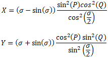
Where P = (β1 + β2)/2 and Q = (β2 - β1)/2
In the expressions above, β1 and β1 are reduced latitudes using the equation below:
tan(β) = (1 - f)tan(ϕ)
where ϕ is the latitude of a point.
Note that neither the haversine formula nor Lambert's formula provides an exact distance because it is not possible to account for every irregularity on the surface of the Earth.
A distance calculator does not measure the space between two objects. It measures the space between two representations of objects—and the gap between those two things is where expensive mistakes hide. Whether you are routing a delivery fleet, calibrating a sensor array, or clustering customer segments, the calculator’s output is only as valid as the coordinate system, metric, and dimensionality you feed it. Pick the wrong assumptions, and two points that look “close” can be operationally distant.
The Hidden Variable: Your Coordinate System Distorts Everything
Most users paste in latitude-longitude pairs without a second thought. That works until it doesn’t. Geographic distance calculators assume a model of Earth’s shape, and models differ.
| Model | Shape Assumed | Error at 1,000 km | Best Use Case |
|---|---|---|---|
| Flat-earth (equirectangular) | Cylinder | Up to ~22% | Sub-kilometer, equatorial regions only |
| Haversine | Sphere | ~0.5% | General-purpose, < 10,000 km |
| Vincenty | Ellipsoid (WGS-84) | ~0.001% | Precision surveying, geodesy |
| Geodesic (Karney) | Ellipsoid, high-order | Negligible | Satellite orbital mechanics |
The trade-off is stark. Haversine executes in microseconds. Karney’s algorithm can require iterative refinement. If you choose Haversine for a transcontinental flight path, you gain speed but accept systematic error that compounds over long arcs—error that shifts north-south routes more than east-west ones because Earth bulges at the equator. Vincenty fails near antipodal points entirely, a documented edge case that crashes some implementations.
For non-geographic data—say, customer feature vectors in R^n—the coordinate system problem mutates. Here, “distance” lives in an abstract space where axes may have incompatible units: dollars, click-through rates, satisfaction scores. Normalization precedes calculation. Skip it, and the variable with largest magnitude dominates regardless of predictive value. Standardization (z-scores) versus min-max scaling produces different nearest-neighbor sets. There is no universal right choice. Min-max preserves zero-points and bounded interpretability; z-scores handle outliers more gracefully but distort relative gaps in dense regions.
EX: Walking Through a Concrete Calculation
Hypothetical example for demonstration purposes.
Two sensors report positions: - Sensor A: φ₁ = 40.7128° N, λ₁ = 74.0060° W (New York) - Sensor B: φ₂ = 51.5074° N, λ₂ = 0.1278° W (London)
We compute great-circle distance via Haversine, then expose where precision matters.
Step 1: Convert to radians - φ₁ = 0.7102 rad, λ₁ = -1.2915 rad - φ₂ = 0.8990 rad, λ₂ = -0.0022 rad
Step 2: Apply Haversine formula
$a = \sin^2\left(\frac{\Delta\phi}{2}\right) + \cos(\phi_1)\cos(\phi_2)\sin^2\left(\frac{\Delta\lambda}{2}\right)$
$c = 2 \cdot \text{atan2}\left(\sqrt{a}, \sqrt{1-a}\right)$
d = R ⋅ c
With Earth radius R = 6,371 km: - Δφ = 0.1888, Δλ = 1.2893 - a = 0.1594 - c = 0.8260 rad - d ≈ 5,586 km
Step 3: Compare to Vincenty
Running the same points through an ellipsoidal calculation yields approximately 5,570 km. The 16 km gap (0.29%) seems trivial until you multiply by fuel burn rates across thousands of flights annually, or until you’re guiding a glide vehicle with limited energy reserve.
Step 4: Euclidean trap in high dimensions
Suppose instead these were 50-dimensional user behavior vectors. The Euclidean distance formula generalizes directly:
$d_{euclidean} = \sqrt{\sum_{i=1}^{n}(x_i - y_i)^2}$
But in high dimensions, relative contrast between nearest and farthest neighbors degrades—distances concentrate. For n > 15, Manhattan distance (L1) often preserves more discriminative signal. The calculator won’t warn you. You must decide.
From Calculation to Decision: What to Run Next
Distance is never the end goal. It feeds a downstream choice. The calculator sits in a toolchain, and your next tool depends on what you learned.
| If your output feeds… | Consider next | Key parameter |
|---|---|---|
| Route optimization | Traveling Salesman solver | Distance matrix symmetry (asymmetric for one-way streets) |
| Clustering | DBSCAN or HDBSCAN | ε-neighborhood threshold; this is your distance cutoff |
| Anomaly detection | Isolation Forest or LOF | Local outlier factor uses k-th nearest neighbor distance |
| Similarity search | Approximate nearest neighbor (ANN) index | Recall-vs-latency trade-off; exact distance often too slow |
The sensitivity-to-outliers problem deserves explicit mention. A single corrupted GPS coordinate—say, a transposed digit producing a point in the Pacific—can distort mean distances, centroid calculations, or nearest-neighbor assignments. Median-based robust estimators exist (e.g., geometric median), but no standard distance calculator implements them. You must preprocess or post-process.
For time-series trajectories, Euclidean distance between entire sequences ignores temporal warping. Dynamic Time Warping (DTW) aligns sequences non-linearly before summing pointwise gaps. The computational cost jumps from O(n) to O(n²), but pattern recognition accuracy often justifies it. If you choose Euclidean for speed, you gain simplicity but lose the ability to match sequences with phase-shifted but structurally identical shapes.
The One Change to Make
Stop treating distance as a passive lookup. Before entering coordinates, explicitly write down: (1) the physical or abstract space these points inhabit, (2) the largest acceptable error for your decision, and (3) whether your downstream algorithm assumes metric properties like symmetry and triangle inequality—because cosine similarity, widely used in text analysis, satisfies none of these, and feeding it into a metric-dependent clustering algorithm yields garbage without transformation. The calculator computes. You govern.
Informational Note
This guide explains mathematical and computational principles for educational purposes. For applications involving navigation safety, financial risk, or medical device positioning, consult domain-specific professionals and validate outputs against certified standards.